Sampling and Quantified Error
You should be skeptical of any headline that says the number of jobs in the United States has changed by fewer than about 105,000 since last month. That’s because the monthly jobs growth estimate has a margin of error of about plus or minus 105,000.16
The New York Times made this point with an interactive graphic, showing how the uncertainty in employment figures can badly mislead us.
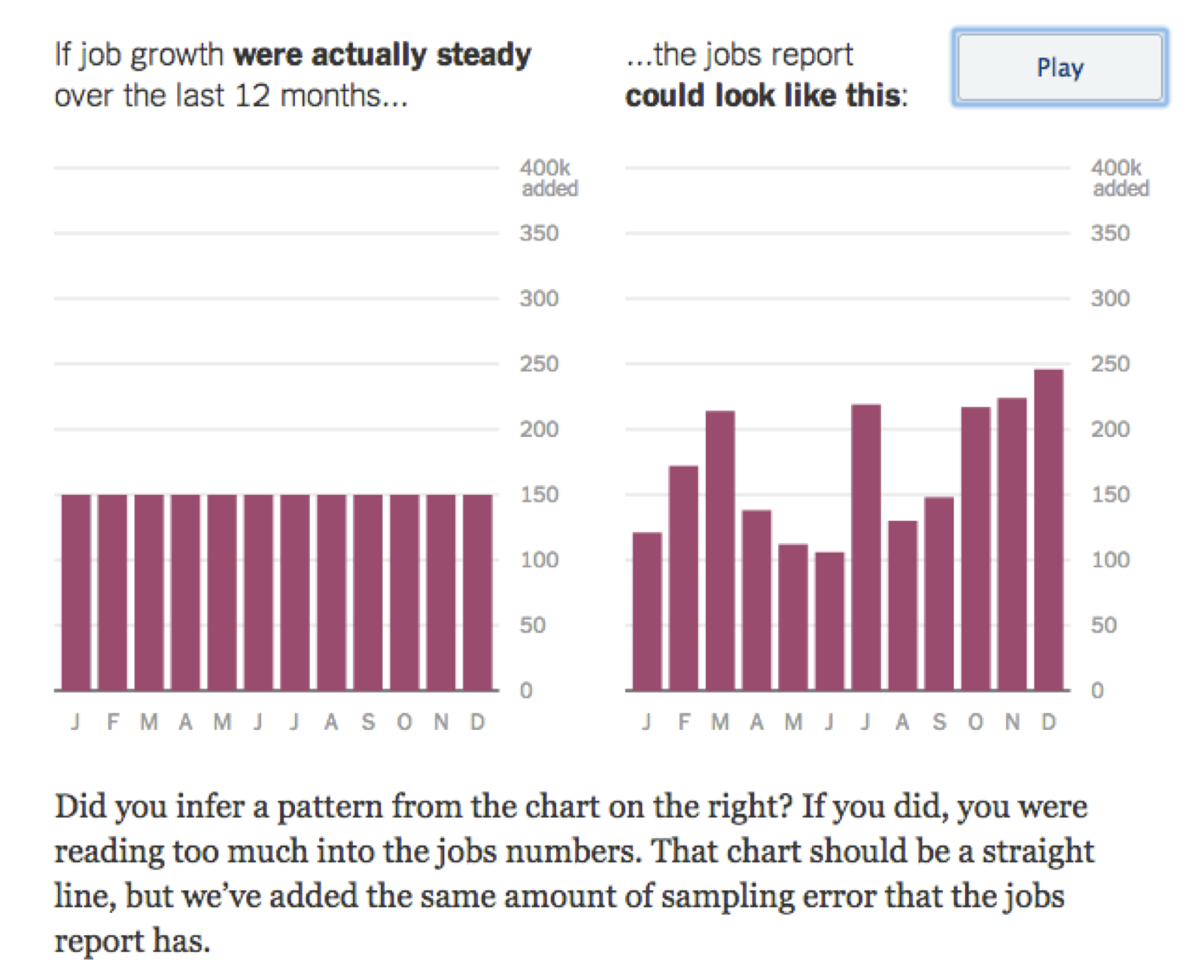
From The New York Times, 2014.17
Here, job growth was consistent at 150,000 new jobs each month, but the released figures show an upward trend just by chance. The unemployment rate calculated by the Bureau of Labor Statistics includes a fair amount of error due to random sampling, up to 105,000 jobs above or below the real value. Pressing “play” animates the right hand chart through endless possible scenarios with the same range of error. If you wait for a minute you can see cases where job growth appears to have any trend you like. Because of these random errors, monthly changes typically mean less than we think they do. Long-term trends are much more reliable.
Political polls also have built-in error. If one candidate is ahead of the other 47 percent to 45 percent, but the margin of error is 5 percent, there is a pretty good chance that another identical poll will show the candidates the other way around. Pretty much any sort of public survey will have intrinsic error, and a reputable source will report the margin of error along with the results. The error of a measurement is a necessary part of understanding what that measurement means.
Maybe you’ve seen formulas for calculating the margin of error for a random sample, but rather than repeat those equations I want to give a sense of why we use random sampling at all and how it leads to quantified error. Expressing how much error there is may seem obvious now, but it was a key innovation in the history of statistics. There is a random sample in the Old Testament: “The people cast lots to bring one out of every ten of them to live in Jerusalem.”vi It couldn't have been long before someone thought of counting by letting each of the chosen stand for 10, but millennia passed before anyone was able to estimate the accuracy of this process.
Sampling is basically a labor-saving device. The unemployment figures need to come out every month, but nobody is going to knock on your door 12 times a year to ask if you have a job. Instead the unemployment rate is calculated from the answers to two surveys: the Current Establishment Survey which samples businesses, and the Current Population Survey which samples households.vii 150,000 randomly chosen people each month,viii each of whom is eventually assigned to one of three categories: “employed,” “unemployed,” or “not in the labor force.”18 The fraction of “unemployed” people among those asked then stands in for the fraction of unemployed people in the whole country.
If this doesn’t strike you as audacious, you’ve probably never thought about just what a poll claims to be able to do. Extrapolating from 150,000 people to 300,000,000 people means collecting information from one person in 2,000 then saying it speaks for the other 1,999. It’s like asking only one person in each neighborhood whether he or she is employed.
Randomness is the key to this, because it makes over-representation by any one group extremely unlikely. It’s possible that all the people who answer a random telephone poll might be unemployed just by chance, giving us a bad estimate. But that will happen rarely—essentially never in practice—and how else should we pick people? We could count through consecutive phone numbers instead, but that might only get us answers from a certain area. Or we could just go through our own contact lists, but that seems even less representative. Randomness is not subject to selection bias precisely because it has no relation to anything else. Even better, although any given sample will give us an estimate that is off by some amount, the most common value is going to be the true value. Also, it’s randomness that allows us to reason about what the error is. Instead of reasoning about the error of a single survey, which is unknowable, we can reason about the error of the sampling process across many different surveys. This is akin to saying that we can’t know what the next roll of the die will be, but there is a one-sixth chance it will be a five.
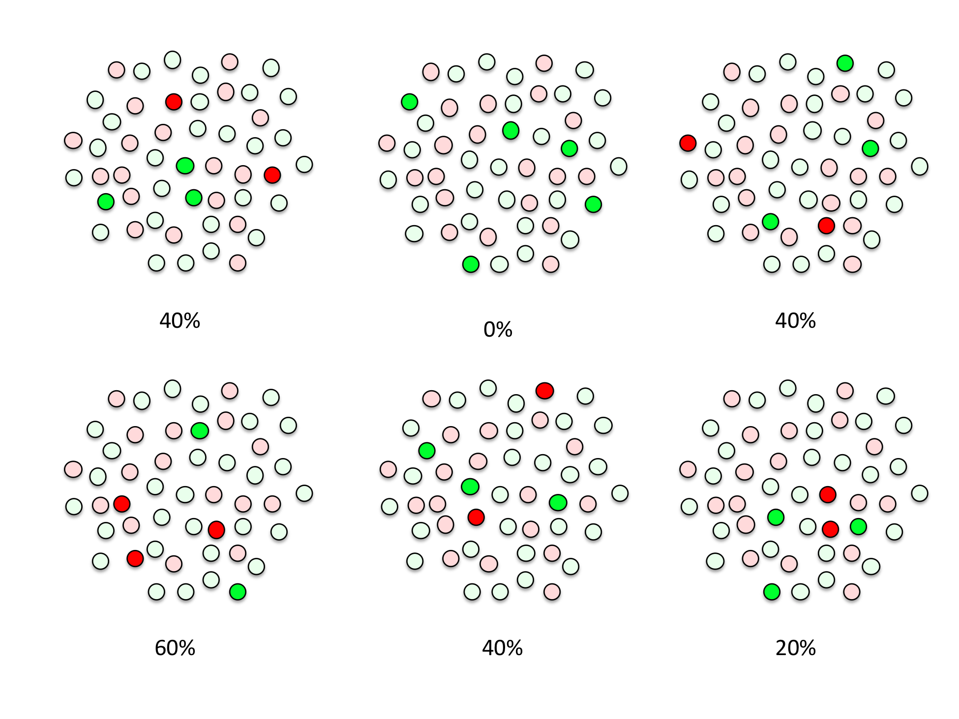
Let’s make the problem a little simpler and imagine that there are only 50 people in the whole country, and you’ve computed the unemployment rate by sampling five of them. You could have ended up with many different sets of five people in your sample had chance taken a different course, but there are a finite number of possibilities. Here are some of them, and the different unemployment rate estimates that each one would give you:
You can imagine drawing a picture of every possible set of names out of 50. You’ll end up with “50 choose 5” different sampling patterns, a number which is usually written  . You can get an actual number for this using the “choose” or “combinations” function of a scientific calculator or programming language, and it’s 2,118,760, over two million. There are an awful lot of ways to pick five random things out of 50 possible things, and a hugely larger number of ways to pick 150,000 people out of 300,0000,000, but we can count with simple formulas either way.
We can group all of these sampling patterns into six piles, according to how many people in each sample turned up unemployed, zero to five. This groups our answers into unemployment rates of 0/5, 1/5, 2/5, 3/5, 4/5, and 5/5, which is the same as 0%, 20%, 40%, 60%, 80%, and 100% unemployment. Because each possible sample—each set of five names—is equally likely, the size of each pile tells you your chances of getting a final estimate with that number of unemployed people. This is the key insight that will allow us to quantify how often we expect our unemployment estimate to be wrong, and by how much.
You don’t actually need stacks of drawings to calculate the error of an unemployment estimate, because we can directly calculate the number of samples of each kind. For example, we can work out how many samples include exactly one unemployed person. Here there are 50 people, 20 of whom are unemployed. The total number of ways to choose five people from 50 so that exactly one turns up unemployed is equal to the number of ways to pick one unemployed person from 20, times the number of ways to pick four unemployed people out of 30.
This is written  using the standard notation for “choose.” Some readers will recognize a similarix term in the binomial distribution function B(50,0.4), the formula developed by Bernoulli some time in the 1680s.
This formula makes it possible to tally the number of ways to get a sample with any particular number of unemployed people. Dividing the number of possible samples for each level of unemployment by the total of 2,118,760 possible samples gives the probability of seeing each possible unemployment estimate.
| Estimated Unemployment | No. Samples | Probability of Getting This Answer |
|---|---|---|
| 0% | 142,506 | 0.07 |
| 20% | 548,100 | 0.26 |
| 40% | 771,400 | 0.36 |
| 60% | 495,900 | 0.23 |
| 80% | 145,350 | 0.07 |
| 100% | 15,504 | 0.01 |
To make this easier to see we can plot the figures like so:
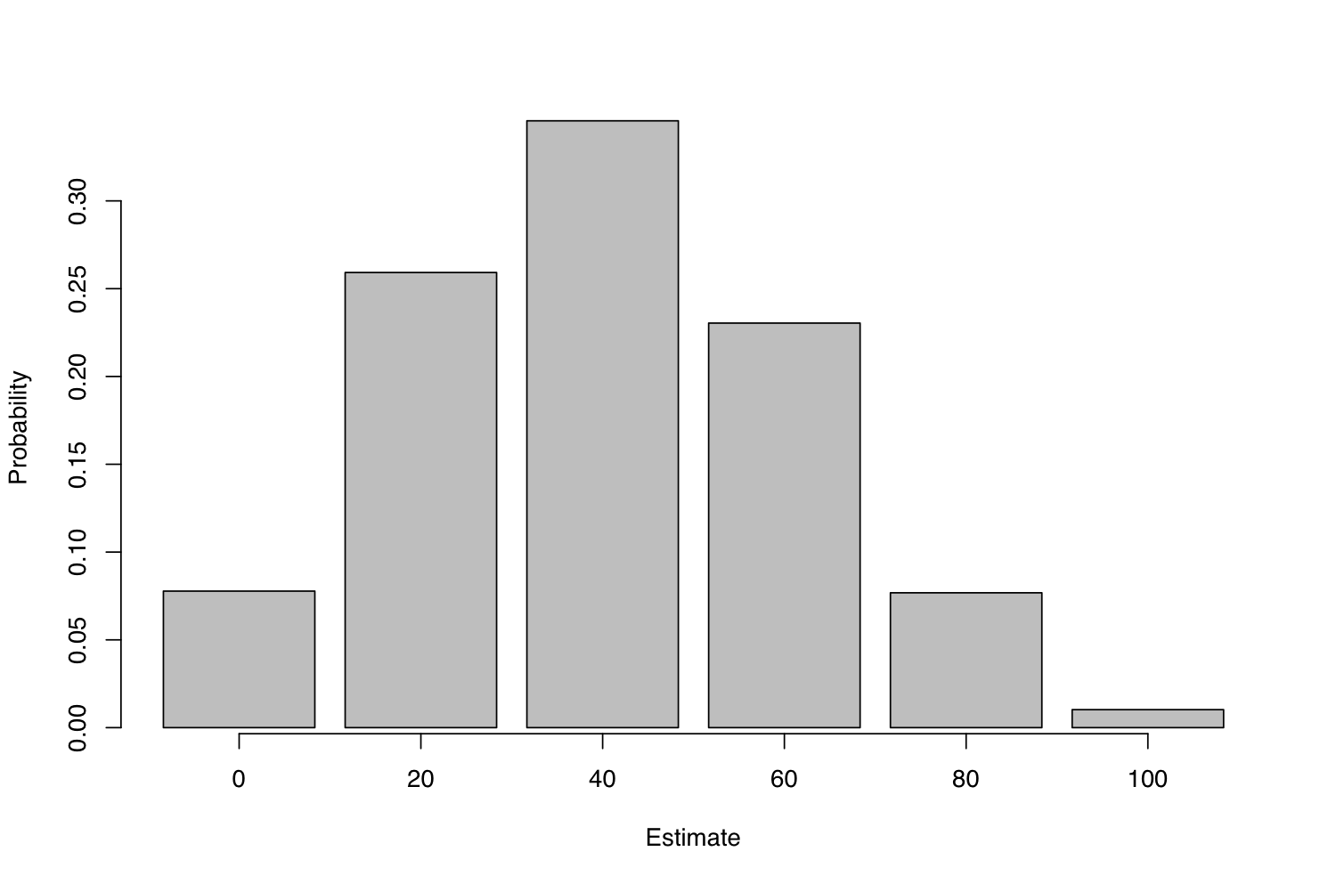
This chart shows a sampling distribution, meaning that we would expect to see each answer in these proportions if we repeated the random sampling process many times. As we had hoped, answers closer to the truth occur more often than those further away, and the most common answer is the correct one. There’s a probability of 0.36, or a 36 percent chance, that we’ll end up with exactly the right answer from our little survey.
This distribution tells us everything we can know about the possible error in our sample value. But we’ll often want a more understandable summary, and one way of summarizing an error distribution is to say how often we’ll get within a certain distance of the correct answer. Let’s say we want to know how often we can expect to get either the true answer of 40%, or the closest incorrect answers of 20% and 60%. This requires adding up the probabilities that we get 20%, 40%, or 60%, which corresponds to seeing one, two, or three unemployed people our sample. There’s a probability of 0.26 + 0.36 + 0.23 = 0.85 that we’ll see any of these three answers.
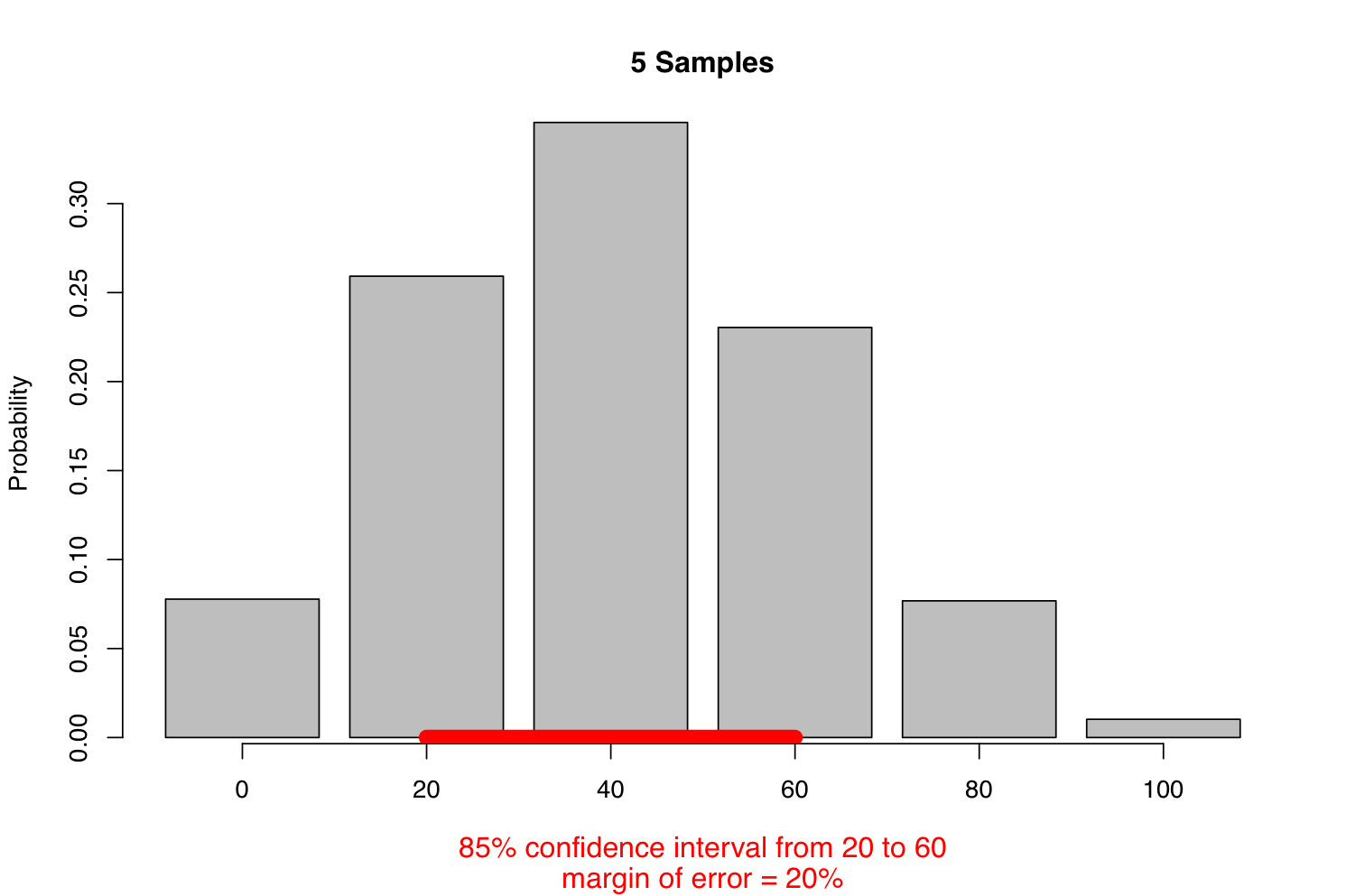
Among the 2,118,760 different samples of five that we could draw from our population of 50 people, we find that 1,815,400 or 85 percent of them contain one, two, or three unemployed people. Put another way, 85 percent of all samples contain between 20% and 60% unemployed.x is known as an 85-percent confidence interval. Because this interval covers a 40% range, and our best estimate is right in the middle, we say that the estimate has a margin of error of 20%. The margin of error is always half of the width of the confidence interval.
We need one more step. So far we’ve been talking about the possible samples we might get for a given true unemployment rate of 40%, and how often we’ll end up with each estimated number. In reality we never get to know the true unemployment rate! We only ever get one sample, and this gives us only a single error-prone estimate. Instead of “how often is the estimate within the margin of error of the true value,” the question we really need to ask is “how often will the true value be within the margin of error of the estimate?”
To do this, we start with the estimated unemployment rate, that is, the rate of unemployment in the actual sample we have. We assume that this is the true rate and construct a margin of error using the process above. If the estimate is within 20% of the true value, then it follows that the true value is within 20% of the estimate. This isn’t perfectly accurate, because the margin of error varies in width depending on the true value, so our estimated margin of error won’t be quite right if the estimate isn’t quite right. You can work out more precise formulas, but this simple method of substituting the estimate for the true value gives a close approximation for practical survey sizes, and it’s widely used in practice.
And that’s it. We’ve now calculated the margin of error on our unemployment estimate. There many different ways of phrasing our result, which all mean the same thing.
The 85-percent confidence interval is 20% to 60%
The answer is 40% with a margin of error of 20%, 17 times out of 20.
We are 85 percent certain that the true answer is between 20% and 60%
The answer is 40% ± 20% at 85 percent confidence.
Notice that we always use two values to measure the uncertainty: a margin of error and the probability that the true answer falls within that margin of error.xi of error, in this case 20% to 60%, is called the 85-percent confidence interval. The 85 percent figure itself is called the confidence level. Whatever language we use, we have quantified the error in our survey in two values: a range of error and how often you’ll see that something within that range.
If 40% ± 20% at an 85-percent confidence level is a precise enough answer, you’ve reduced your work by a factor of 10 by asking only five out of 50 people. If it’s not precise enough, you can sample more people. To compare the error distributions of different numbers of samples, it helps to hold the confidence level constant. The Bureau of Labor Statistics reports the margin of error on unemployment figures at the 90-percent level, so we will too. We’ll also do the calculations as if we’re sampling from a real country’s population, which is much larger than 50.
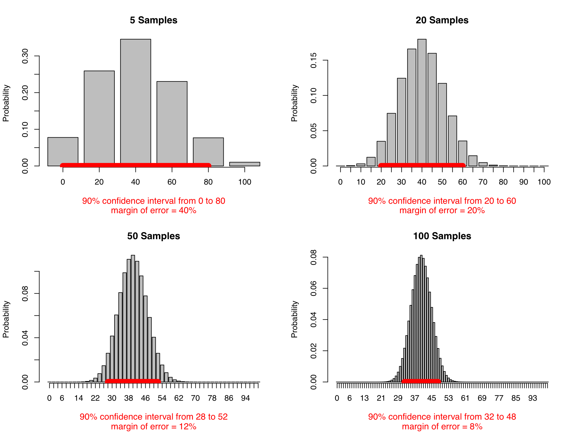
The accuracy gets better as you ask more people. As the number of samples gets larger—we’re up to 100 in the last picture above—the margin of error gets narrower (for a particular confidence level) and the distribution of possible answers rapidly approaches the classic bell-shaped curve, the normal distribution. Even better, for large samples the error caused by sampling depends primarily the sample size, not the population size. This means that estimating the opinions of a hundred million people takes barely more work than estimating the opinions of one million. By the time you survey 1,000 people, the margin of error is down to 3% at the 90-percent confidence level.
This is how we know the error in our monthly unemployment estimates. The Current Population Survey samples 150,000 people out of 300,000,000. The Bureau of Labor statistics has run the math and worked out that it’ll get within 300,000 of the true unemployment rate 90 percent of the time, which corresponds to 0.2% difference in the national unemployment rate.19 The 300,000 is the margin of error and the 90 percent is the confidence level.
If a 90-percent confidence interval sounds like a 10 percent chance of disaster, we can trade off between the estimated error and the risk of falling outside of that error: it’s equally true to say that 99 percent of the time the unemployment figures will be accurate to within ± 0.3%. This is the same thing, reported differently; we’re just widening the red line on the above charts until it covers 99 percent of the possible outcomes.
There is an intricate bargain being struck here. In exchange for a little fuzziness (the margin of error) and a little risk (the confidence level) we’ve reduced our work to calculate the unemployment rate by 2,000 times. This remains astonishing to me. it’s beautiful and non-obvious and took millennia for humanity to see it.